

Styling
For both vector and raster data, eodash uses a shared JSON style definition with use of OpenLayers flat style and JSON Form definition language as extended by the EOxElement eox-jsonform and eox-layercontrol-legend
Vector styling
Basic example:
{
    "fill-color": "red",
    "stroke-color": "black",
    "stroke-width": 1
}
Changing style UI
You can add user controls by combining style variables with JSON Form. Example of adjustable stroke width:
{
    "variables": {
        "strokeWidth": 1
    },
    "fill-color": "red",
    "stroke-color": "black",
    "stroke-width": ["var", "strokeWidth"],
    "jsonform": {
        "type": "object",
        "title": "Data configuration",
        "properties": {
          "strokeWidth": {
            "type": "number",
            "minimum": 0,
            "maximum": 10,
            "format": "range",
            "default": 0
          }
        }
    }
}
The name of variable strokeWidth must match in variables object, variable inside the flatstyle properties (stroke-width), and jsonform.properties.
Tips and tricks
Taking these concepts into account, one can extend the style to use also the get functionality of flat styles to access feature properties of the geoJSON and encoded expressions truly custom and interactive styles can be created.
There are a few interesting tricks for properties, which "somehow do not fit".
Convert numbers to strings: to-string or concat:
"text-value": ["to-string", ["get", "numberproperty"]],
"text-value": ["concat", ["get", "numberproperty"], "somestring, e.g. unit of measurement"],
If a property is null, styling may fail. Use coalesce:
Therefore if the feature property is null it will return "N/A" in this case
"text-value": ["to-string",["coalesce", ["get", "propertywithsomenullvalues"], "N/A"]],.
Nested properties:
{
   "text-value":[
      "to-string",
      [
         "coalesce",
         [
            "get",
            "topproperty",
            "subproperty",
            "subsubproperty"
         ],
         "N/A"
      ]
   ]
}
Other examples
Example of color range applied to style Ice charts data according to the Sea Ice Concentration percentage with values 0-100.
{
  "tooltip": [{"id": "CT", "title": "CT"}],
  "fill-color": [
    "case",
    ["!", ["get", "CT"]],
    [0, 0, 0, 0],
    ["<", ["get", "CT"], 0],
    [0, 0, 255, 0],
    ["<=", ["get", "CT"], 10],
    [150, 200, 255, 1],
    ["<=", ["get", "CT"], 40],
    [140, 255, 159, 1],
    ["<=", ["get", "CT"], 70],
    [255, 255, 0, 1],
    ["<=", ["get", "CT"], 90],
    [255, 125, 7, 1],
    ["<=", ["get", "CT"], 100],
    [255, 0, 0, 1],
    [0, 0, 255, 1]
  ],
  "stroke-color": "black",
  "stroke-width": 1
}
Hidden fields
You can hide fields via "options": {"hidden": true},to create "composed" fields to be later reused in the styles.
In this example a tooltip content is created from a hidden field, which is a composite of values from three other selection fields ship_class, type_of_ice and type_of_visualization via a watch syntax. Also see enum_titles property for human readable labels of fields.
{
    "jsonform": {
        "type": "object",
        "title": "Data configuration",
        "properties": {
            "type_of_visualisation": {
                "title": "Type of Visualisation",
                "type": "string",
                "enum": [
                    "airss",
                    "WMO Concentration"
                ],
                "options": {
                    "enum_titles": [
                        "AIRSS Ice Numeral Go/No Go",
                        "WMO Concentration"
                    ]
                },
                "default": "airss"
            },
            "ship_class": {
                "title": "Ship Class",
                "type": "string",
                "enum": [
                    "type_a",
                    "type_b",
                    "type_c",
                    "type_d",
                    "type_e",
                    "type_cac3",
                    "type_cac4"
                ],
                "options": {
                    "enum_titles": [
                        "Type A",
                        "Type B",
                        "Type C",
                        "Type D",
                        "Type E",
                        "Type CAC3",
                        "Type CAC4"
                    ]
                },
                "default": "type_a"
            },
            "type_of_ice": {
                "title": "Type of Ice (decayed/standard)",
                "type": "string",
                "enum": ["standard", "ridged"],
                "default": "standard"
            },
            "combined_prop": {
                "type": "string",
                "template": "{{vis}}_{{ice}}_{{ship}}_go_no_go",
                "options": {"hidden": true},
                "watch": {
                    "vis": "type_of_visualisation",
                    "ice": "type_of_ice",
                    "ship": "ship_class"
                }
            }
        }
    },
    "tooltip": [
        {"id": "wmo_concentration", "title": "WMO Concentration"},
        {"id": "wmo_stage_of_development", "title": "Stage of development"},
        {
            "id": "{{combined_prop}}",
            "title": "AIRSS value (ship class: {{ship_class}} ice: {{type_of_ice}})"
        }
    ],
    "variables": {
        "ship_class": "type_a",
        "type_of_ice": "standard",
        "type_of_visualisation": "airss",
        "combined_prop": "airss_standard_type_a_go_no_go"
    },
    "fill-color": [
        "case",
        ["==", ["var", "type_of_visualisation"], "WMO Concentration"],
        [
            "match",
            ["get", "wmo_concentration"],
            "Ice Free",
            [0, 100, 255, 1],
            "Open Water (< 1/10 ice)",
            [150, 200, 255, 1],
            "Bergy Water",
            [150, 200, 255, 1],
            "1/10 - 3/10",
            [140, 255, 160, 1],
            "4/10 - 6/10",
            [255, 255, 0, 1],
            "7/10 - 8/10",
            [255, 125, 5, 1],
            "9/10 - 10/10",
            [255, 0, 0, 1],
            "8/10 - 9/10",
            [255, 0, 0, 1],
            "8/10 - 10/10",
            [255, 0, 0, 1],
            "7/10 - 9/10",
            [255, 125, 7, 1],
            "6/10 - 7/10",
            [255, 125, 7, 1],
            "5/10 - 7/10",
            [255, 255, 0, 1],
            "3/10 255 5/10",
            [255, 255, 0, 1],
            "3/10 255 4/10",
            [255, 255, 0, 1],
            "2/10 255 4/10",
            [255, 255, 0, 1],
            "Unknown/Undetermined",
            [255, 255, 255, 1],
            [255, 255, 255, 1]
        ],
        ["==", ["var", "type_of_visualisation"], "airss"],
        [
            "case",
            ["==", ["get", "polygon_type"], "Ice Free"],
            [0, 100, 255],
            ["==", ["get", ["var", "combined_prop"]], "<= 0 IN < 2"],
            [217, 239, 139, 1],
            ["==", ["get", ["var", "combined_prop"]], "<= 2 IN < 5"],
            [166, 217, 106, 1],
            ["==", ["get", ["var", "combined_prop"]], "<= 5 IN < 10"],
            [102, 189, 99, 1],
            ["==", ["get", ["var", "combined_prop"]], "IN > 10"],
            [26, 152, 80, 1],
            ["==", ["get", ["var", "combined_prop"]], "<= -2 IN < 0"],
            [255, 135, 135, 1],
            ["==", ["get", ["var", "combined_prop"]], "<= -5 IN < -2"],
            [255, 82, 82, 1],
            ["==", ["get", ["var", "combined_prop"]], "<= -10 IN < -5"],
            [255, 0, 0, 1],
            [0, 0, 0, 1]
        ],
        [0, 0, 0, 1]
    ],
    "stroke-color": "black",
    "stroke-width": 1
}
Raster styling
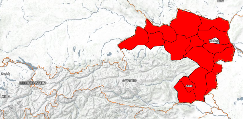
Here is a more complex example which shows the use of ["band", 1] to access values from two single band COGs, normalizing the data to 0-1 values, and then applying an interpolated 16-value viridis colormap. The vmin and vmax variables are used to perform the normalization allowing dynamic color range adaptation in the eodash instance.
Band 2 is used to filter what data gets rendered. If the case does not apply, it renders the corresponding pixel as transparent.
Additionally, a dynamic legend is defined by using the domainProperties referencing the jsonform and style variables vmin and vmax. These properties can be named differently for other datasets, but must end with min and max. Hex color code (#ff00ff) strings can be used, too, for both legend and color.
{
    "variables": {
      "vmin": 2,
      "vmax": 5,
      "settlementDistance": 0
    },
    "color": [
        "case",
        [
            "all",
            [">", ["band", 1], 1],
            [">=", ["band", 2], ["var", "settlementDistance"]]
        ],
        [
            "interpolate",
            ["linear"],
            ["/", ["-", ["band", 1], ["var", "vmin"]], ["-", ["var", "vmax"], ["var", "vmin"]]],
            0, [68, 1, 84, 1],
            0.067, [70, 23, 103, 1],
            0.133, [71, 44, 122, 1],
            0.2, [65, 63, 131, 1],
            0.266, [59, 81, 139, 1],
            0.333, [52, 97, 141, 1],
            0.4, [44, 113, 142, 1],
            0.467, [39, 129, 142, 1],
            0.533, [33, 144, 141, 1],
            0.6, [39, 173, 129, 1],
            0.666, [66, 187, 114, 1],
            0.733, [92, 200, 99, 1],
            0.8, [131, 210, 75, 1],
            0.867, [170, 220, 50, 1],
            0.933, [212, 226, 44, 1],
            1, [253, 231, 37, 1]
        ],
        [
        "color", 0, 0, 0, 0
        ]
    ],
    "legend": {
        "title": "[kWh/m²/day]",
        "range": [
            "rgba(68, 1, 84, 1)",
            "rgba(70, 23, 103, 1)",
            "rgba(65, 63, 131, 1)",
            "rgba(59, 81, 139, 1)",
            "rgba(52, 97, 141, 1)",
            "rgba(44, 113, 142, 1)",
            "rgba(39, 129, 142, 1)",
            "rgba(33, 144, 141, 1)",
            "rgba(39, 173, 129, 1)",
            "rgba(66, 187, 114, 1)",
            "rgba(92, 200, 99, 1)",
            "rgba(131, 210, 75, 1)",
            "rgba(170, 220, 50, 1)",
            "rgba(212, 226, 44, 1)",
            "rgba(253, 231, 37, 1)"
        ],
        "domainProperties": ["vmin", "vmax"]
    },
    "jsonform": {
      "type": "object",
      "title": "Data configuration",
      "properties": {
        "settlementDistance": {
            "type": "number",
            "minimum": 0,
            "maximum": 5000,
            "format": "range",
            "default": 0
        },
        "vminmax": {
          "title": "Global horizontal irradiation",
          "description": "[kWh/m²/day]",
          "type": "object",
          "properties": {
            "vmin": {
              "type": "number",
              "minimum": 0,
              "maximum": 5,
              "format": "range",
              "default": 2
            },
            "vmax": {
              "type": "number",
              "minimum": 0,
              "maximum": 5,
              "format": "range",
              "default": 5
            }
          },
          "format": "minmax"
        }
      }
    }
  }
Here is how that translates to a visualization in the eodash instance (without the legend):
Controlling which bands to use via UI
Style variables and jsonform can be used to let user switch between bands or data properties.
The following style allows accessing 6 hourly predictions of Ice drift from Sentinel-1 scenes over the same area of interest and adapting color stretch:
{
    "legend": {
        "title": "S1 Scene",
        "range": [
            "rgba(0, 0, 0, 1)",
            "rgba(255, 255, 255, 1)"
        ],
        "domainProperties": ["vmin", "vmax"]
    },
    "variables": {
        "vmin": 0,
        "vmax": 1000,
        "prediction_hour": 1
    },
    "color": [
        "case",
        [">", ["band", ["var", "prediction_hour"]], 0],
        [
            "interpolate",
            ["linear"],
            [
                "/",
                ["-", ["band", ["var", "prediction_hour"]], ["var", "vmin"]],
                ["-", ["var", "vmax"], ["var", "vmin"]]
            ],
            0,
            [0, 0, 0, 1],
            1,
            [255, 255, 255, 1]
        ],
        ["color", 0, 0, 0, 0]
    ],
    "jsonform": {
        "type": "object",
        "title": "Data configuration",
        "properties": {
            "prediction_hour": {
                "type": "number",
                "minimum": 1,
                "maximum": 6,
                "step": 1,
                "format": "range",
                "default": 1
            },
            "vminmax": {
                "title": "S1 warped predictions",
                "type": "object",
                "properties": {
                    "vmin": {
                        "type": "number",
                        "minimum": 0,
                        "maximum": 3000,
                        "format": "range",
                        "default": 0
                    },
                    "vmax": {
                        "type": "number",
                        "minimum": 0,
                        "maximum": 3000,
                        "format": "range",
                        "default": 1000
                    }
                },
                "format": "minmax"
            }
        }
    }
}